Sample Explorations
Annotated examples showing what makes a strong IB Math exploration
Scoring Overview
| Summary | Sample | A | B | C | D | E(SL) | E(HL) | SL | HL |
|---|---|---|---|---|---|---|---|---|---|
| Acceptable | Car Windows and Angles | 2 | 2 | 1 | 1 | 2 | 1 | 8 | 7 |
| Good | The A-Pillar Blind Spot | 3 | 2 | 2 | 2 | 4 | 3 | 13 | 12 |
| Excellent SL | Coming Soon | - | - | - | - | - | - | - | - |
| Excellent HL | Coming Soon | - | - | - | - | - | - | - | - |
Car Windows and Angles
Introduction
Ever since I was young, I've been fascinated by cars and automotive engineering. My dad used to take me to car shows every summer, and I remember being absolutely amazed by all the different designs and models on display. I've always loved looking at the sleek curves of sports cars, the rugged build of SUVs, and the compact efficiency of city cars. The variety in automotive design is truly remarkable. When I was about 10, my uncle bought a brand new Mercedes-Benz, and I remember sitting in the driver's seat (while parked, of course!) and pretending to drive it. The interior was so luxurious with leather seats and a high-tech dashboard with all sorts of digital displays. That experience really sparked my interest in automotive design and how cars are built. I started reading car magazines and watching documentaries about car manufacturing. I found it fascinating how engineers have to balance so many different factors - safety, efficiency, aesthetics, cost, and functionality.
Over the years, I've noticed various features of car design that I find interesting and I've thought about them a lot. For instance, I've wondered why windscreens are angled the way they are, why some cars have bigger side mirrors than others, and why the metal frames around windows vary so much in thickness between different models and different manufacturers. I particularly noticed that in my mum's car, there's this thick metal bar between the front windscreen and the side window - I later learned through my research that this is called the A-frame or A-pillar. Sometimes when I'm sitting in the passenger seat, this bar blocks my view of things on the side of the road, like pedestrians crossing or cyclists. I thought this might be worth investigating mathematically using geometry and trigonometry and maybe some other mathematical techniques. For this essay my teacher suggested I look into angles so that's what I will do.
I think that investigating the A-frame could be really interesting because it combines practical real-world engineering with mathematics. I'll probably need to use angles and triangles and things like that to work out the blind spot. My aim is to investigate A-frames and blind spots in cars and see what I can find out about them and maybe it will help with my understanding of engineering, which I am interested in studying at university.
Background Research
The A-frame, which is also sometimes called the A-pillar, is the vertical support structure on either side of the windscreen in a car. It's called the A-frame because it's the first pillar when you count from the front to the back of the car (there are also B-pillars and C-pillars which come after the A-frame). According to my research that I did online on various websites, these A-frame pillars are really essential and important for the structural integrity of the car. The A-frames need to be strong enough to support the roof of the car, especially in the event of a rollover accident where the car might flip over. This is really important for safety.
This creates a design challenge for car manufacturers: thicker pillars are safer because they're stronger but they create larger blind spots for the driver, while thinner pillars give better visibility and smaller blind spots but they might compromise the safety aspect because they're not as strong. So there's a trade-off between the two competing factors of safety and visibility. Car designers have to think about both of these things when they design the A-frame.
For the mathematics, I will use basic trigonometry to calculate angles. The main formula I will use is SOHCAHTOA and the cosine or sine rule
Data Collection
I measured the A-frame width and my eye distance in my family car (a 2018 Honda Civic).
Measurements:
- A-frame width: 12 cm
- Distance from eye to A-frame: 95 cm
Calculations
I drew a diagram of the situation (see Figure 1).
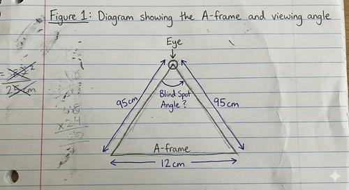
Looking at my diagram, I can see that the A-frame and my eye form a triangle. The A-frame is 12cm wide and I'm sitting 95cm away from it. I think this is an isosceles triangle because the distances to each side of the A-frame are roughly equal.
To find the angle, I will use the cosine rule. The cosine rule says:
$$c^2 = a^2 + b^2 - 2ab\cos(C)$$
In my triangle:
- $a$ = distance from eye to left edge = 95 cm
- $b$ = distance from eye to right edge = 95 cm
- $c$ = width of A-frame = 12 cm
- $C$ = the blind spot angle I want to find
Substituting into the formula:
$$12^2 = 95^2 + 95^2 - 2(95)(95)\cos(C)$$
$$144 = 9025 + 9025 - 18050\cos(C)$$
$$144 = 18050 - 18050\cos(C)$$
$$18050\cos(C) = 18050 - 144$$
$$\cos(C) = \frac{17906}{18050}$$
$$\cos(C) = 0.9920$$
$$C = \cos^{-1}(0.9920)$$
$$C = 7.24°$$
So the blind spot angle is approximately 7.2 degrees.
I wondered what would happen if I moved my head forward or backward. If I lean forward to 85cm from the A-frame:
$$12^2 = 85^2 + 85^2 - 2(85)(85)\cos(C)$$
$$144 = 14450 - 14450\cos(C)$$
$$\cos(C) = \frac{14306}{14450} = 0.9900$$
$$C = 8.1°$$
And if I lean back to 105cm:
$$\cos(C) = \frac{22000}{22050} = 0.9977$$
$$C = 6.6°$$
So if you move closer to the A-frame the blind spot gets bigger, and if you move further away it gets smaller.
| Distance from A-frame (cm) | Blind spot angle (degrees) |
|---|---|
| 85 | 8.1 |
| 95 | 7.2 |
| 105 | 6.6 |
Conclusion
My investigation found that the A-frame in a Honda Civic creates a blind spot of approximately 7.2 degrees when viewed from the driver's position. The blind spot angle decreases as you move further from the A-frame, but not in a linear way.
This investigation could be useful for car designers who need to balance safety (thick pillars) with visibility (thin pillars).
Limitations
My investigation has several limitations:
- I only measured one car - different models might have different A-frame widths
- I didn't account for the angle of the A-frame (it's not perfectly vertical)
- I assumed everyone sits at the same distance from the A-frame
- I didn't measure the A-frame thickness at different heights (it might taper)
If I were to do this investigation again, I would measure multiple cars and try to create a formula that predicts blind spot size based on A-frame width and seating position.
What I Learned
I learned that you can use simple trigonometry to solve real-world problems. I was surprised that the relationship between distance and angle wasn't linear - I expected it to decrease at a constant rate. I also learned that A-frames are thicker than I thought (12cm is quite substantial) and that even this creates a significant blind spot of over 7 degrees.
The hardest part of this investigation was making accurate measurements with a ruler in the car - it was difficult to measure the exact distance from my eye to the A-frame because I couldn't hold the ruler and sit in a natural position at the same time.
The A-Pillar Blind Spot: How Much of the Road Can't You See?
Introduction and Aim
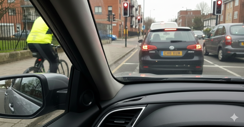
I'm learning to drive, and my instructor keeps telling me to "check properly at junctions." Last week, while waiting to turn, a cyclist seemed to appear from nowhere on my left—I was focusing on the road ahead and they'd come from a hidden spot behind the A-pillar. The image below shows what I mean: the A-pillar is the vertical strip of metal between the windscreen and side window that holds the roof up.
This got me thinking—I could probably use some geometry to work out how large the blind spot actually is, and how it changes with distance. That's what this exploration is about.
Part 1: Setting Up the Geometry
I parked my car safely at home and took measurements to model the blind spot geometry:
[Diagram: Top-down view showing eye position O, A-pillar edges A and B]
Measurements: OA = distance to far edge, OB = distance to near edge, AB = pillar width
- A-pillar width: $AB = 12$ cm
- Distance from eye to near edge of A-pillar: $OB = 60$ cm
- Distance from eye to far edge of A-pillar: $OA = 68$ cm
- Distance from car to pavement edge: approximately 2.5 m when parked
Important assumption: My eye is not equidistant from both edges of the A-pillar—it's closer to the near edge (B). This means the triangle formed is not isosceles, so I cannot simply use $\tan(\theta/2) = \frac{w/2}{d}$. However, since the difference is small (60 cm vs 68 cm), I will first calculate using the cosine rule for accuracy, then check whether the simpler approximation gives similar results.
Using the cosine rule to find the blind spot angle $\theta$:
$$AB^2 = OA^2 + OB^2 - 2 \cdot OA \cdot OB \cdot \cos(\theta)$$
$$12^2 = 68^2 + 60^2 - 2(68)(60)\cos(\theta)$$
$$144 = 4624 + 3600 - 8160\cos(\theta)$$
$$\cos(\theta) = \frac{8080}{8160} = 0.990$$
$$\theta = \cos^{-1}(0.990) = 8.1°$$
The blind spot angle is approximately 8.1°. But this angle alone doesn't tell us much—the key question is: what width of pavement does this obscure at various distances?
Part 2: Blind Spot Width at Distance
The critical insight is that the blind spot widens with distance. Using similar triangles, I can find the width of the hidden region at any distance from my eye.
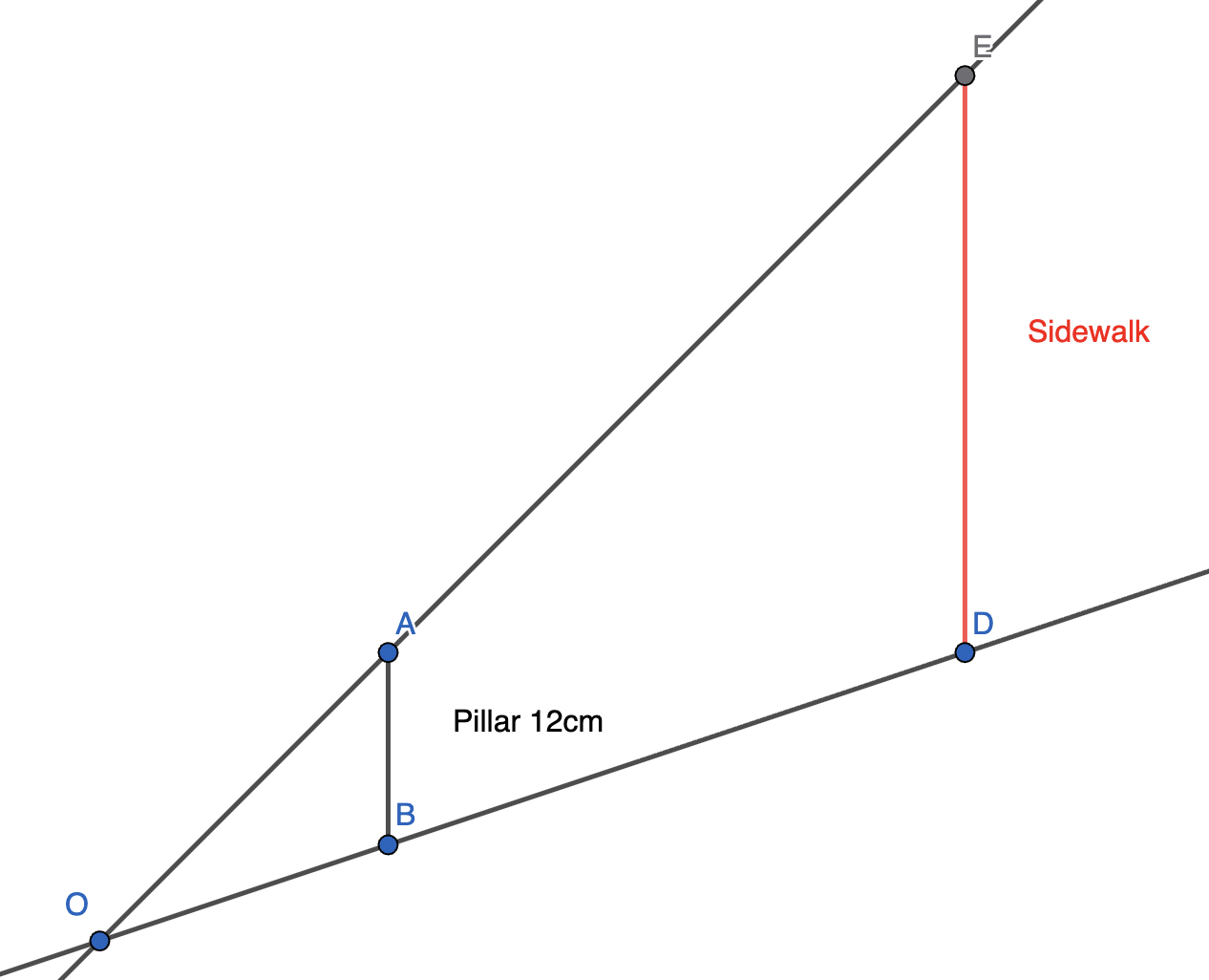
Lines from O through A and B intersect the sidewalk at E and D. Since triangles OAB and OED are similar:
$$\frac{DE}{AB} = \frac{OD}{OB}$$
With $AB = 12$ cm and $OB = 60$ cm (measured from my eye to the near edge of the pillar), if the sidewalk is at distance $OD$ from my eye:
$$DE = \frac{AB \times OD}{OB} = \frac{12 \times OD}{60} = 0.2 \times OD$$
Applying this to realistic distances (measured while safely parked):
| Distance $OD$ (m) | Blind Spot $DE$ (cm) | What this means |
|---|---|---|
| 2.5 (kerb from parked car) | 50 | Could obscure a child |
| 5 (near side of road) | 100 | An adult's full body width |
| 8 (pedestrian crossing) | 160 | A person completely hidden |
| 12 (far side of crossing) | 240 | Multiple pedestrians hidden |
These results are sobering. At a pedestrian crossing distance of 8 metres (typical when stopped at traffic lights), the blind spot is 160 cm wide—enough to completely hide an adult standing still. This explains why cyclists and pedestrians can seem to "appear from nowhere."
Graphical Analysis
I plotted the relationship $DE = 0.2 \times OD$ to visualise how the blind spot grows:
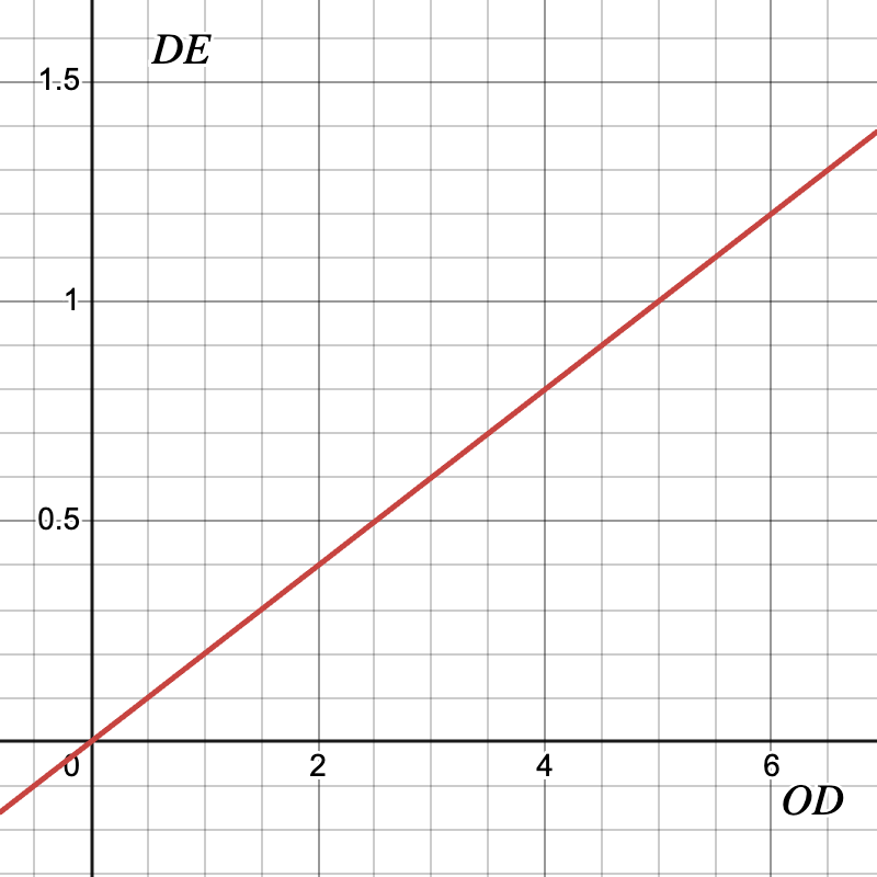
The gradient $\frac{AB}{OB} = \frac{12}{60} = 0.2$ tells us that for every metre of distance, the blind spot grows by 20 cm. The linearity is significant: there is no "safe" distance where the blind spot stops growing. This is an inherent property of similar triangles.
Part 3: Can Head Movement Help?
Drivers are taught to "rock" their head to check A-pillar blind spots. I decided to model this using GeoGebra, which allowed me to create an interactive diagram where I could adjust the head position.
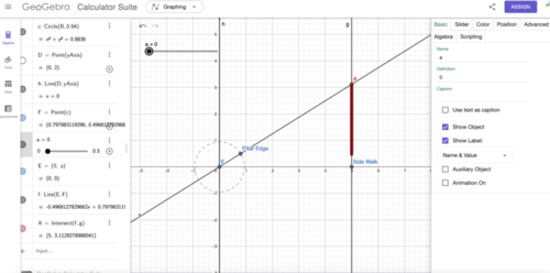
I set up the model with the eye at the origin, the pillar edge at approximately 1 unit (representing ~1 metre in scale), and the sidewalk at $x = 5$. The line from E through the pillar edge intersects the sidewalk, and the red segment A shows the blind spot region.
By adjusting the slider, I found that moving the head position by a small amount significantly reduced the blind spot. The red points trace how the visible region changes as the head moves laterally.
This confirms that the "head rock" technique is effective—even a small lateral movement can reveal objects hidden behind the A-pillar.
Part 4: Assumptions and Limitations
My model assumes a stationary scenario (stopped at traffic lights), which simplifies the mathematics considerably.
Key assumptions:
- The A-pillar is modelled as a flat vertical strip (in reality, it has depth and angle)
- I used $OB$ (distance to near edge) for the similar triangles calculation—using $OA$ would give slightly different results
- The driver's eye is a single point (binocular vision provides some help in practice)
- Objects and vehicle are stationary (a moving pedestrian might enter and exit the blind spot)
I verified the model by sitting in the car (parked safely) and checking whether objects at known distances were hidden as predicted. A traffic cone at 5 metres was indeed mostly obscured, and approximately 2 cm of head movement revealed it. This gives me confidence that the simplified model captures the essential geometry.
Extension Possibilities
This exploration could be extended by considering dynamic scenarios: if a car is moving, the blind spot "sweeps" across the road. A pedestrian walking at constant speed could remain hidden in the blind spot if their velocity matches the sweep rate. Modelling this would require rates of change and parametric equations—perhaps material for a future investigation.
Conclusion
Using the cosine rule and similar triangles, I have shown that the A-pillar creates a blind spot that grows linearly with distance: $DE = 0.2 \times OD$. At typical pedestrian crossing distances (5-10 m), this blind spot is 100-200 cm wide—enough to hide an adult entirely.
Small head movements (1-2 cm) are sufficient to reveal distant objects, validating standard driving advice. However, the model reveals a limitation: for very close objects, the required head movement becomes impractically large, and moving the head towards the pillar actually makes things worse.
The linear model with its acknowledged assumptions provides useful insight into A-pillar safety, though dynamic analysis would be needed for a complete understanding of blind spot hazards while driving.
Dynamic Blind Spot Analysis: How Long Should I Check?
Introduction
I'm learning to drive, and my instructor keeps telling me to "check properly at junctions." Last week, while waiting to turn, a cyclist seemed to appear from nowhere on my left—I was focusing on the road ahead and they'd come from a hidden spot behind the A-pillar. The image below shows what I mean: the A-pillar is the vertical strip of metal between the windscreen and side window that holds the roof up.
When I got home, I sat in our car and experimented. I put a water bottle on the driveway and moved my head side to side, watching it appear and disappear behind the pillar. I realised the blind spot isn't fixed—it moves as I move. This got me thinking: I could probably use some mathematics to figure out how dangerous this actually is.
This exploration investigates three connected questions:
- How large is the blind spot, and how does it grow with distance?
- How long does a moving pedestrian or cyclist spend hidden?
- How long should I pause and actively check before turning?
Part 1: The Geometry of Vision
Setting Up the Model
I'll use a coordinate system with my eye at origin O. The A-pillar has width $w$ = 12 cm (measured in my car), with edges at points A and B. A pedestrian stands at distance $d$ from my eye, somewhere along the line of sight.
Figure 2: The blind spot geometry (not to scale)
The key insight is that the blind spot at distance $d$ depends on the ratio of distances. Using similar triangles:
$$\frac{DE}{AB} = \frac{OD}{OB}$$
Where:
- $OB$ = 60 cm (distance from eye to pillar, measured)
- $AB$ = 12 cm (pillar width, measured)
- $OD$ = distance to pedestrian
- $DE$ = blind spot width at that distance
Rearranging:
$$DE = \frac{AB \times OD}{OB} = \frac{12 \times OD}{60} = 0.2 \times OD$$
So the blind spot width is 20% of the distance to the target. At 5 metres, the blind spot is 1 metre wide. At 10 metres, it's 2 metres wide.
The Angle Calculation
The blind spot width grows with distance, but the angle blocked by the pillar stays constant—it's determined by the pillar geometry, not the target distance. I wanted to calculate this angle using the cosine rule for triangle OAB:
$$AB^2 = OA^2 + OB^2 - 2 \cdot OA \cdot OB \cdot \cos(\theta)$$
With $OA$ = 68 cm, $OB$ = 60 cm, $AB$ = 12 cm:
$$144 = 4624 + 3600 - 8160\cos(\theta)$$
$$\cos(\theta) = \frac{8080}{8160} = 0.990$$
$$\theta = 8.1°$$
This 8.1° angle is significant—it's roughly the width of four fingers held at arm's length. Not huge, but enough to hide a person completely.
Part 2: The Effect of Pillar Width
Different vehicles have different A-pillar widths. Sports cars might have 10 cm pillars; SUVs and trucks can have 18-20 cm for structural rigidity. How does this affect the blind spot?
Interactive Graph: Pillar Width Comparison
Family of functions showing blind spot width vs distance for different A-pillar widths (10cm, 12cm, 15cm, 20cm)
DESMOS/GEOGEBRA PLACEHOLDERFigure 2: Blind spot width vs distance for different A-pillar widths
The graph reveals something striking:
| Pillar Width | Distance to Hide Adult (1.8m) | Distance to Hide Child (0.5m) |
|---|---|---|
| 10 cm | 10.8 m | 3.0 m |
| 12 cm | 9.0 m | 2.5 m |
| 15 cm | 7.2 m | 2.0 m |
| 20 cm | 5.4 m | 1.5 m |
Reflection: My car's 12 cm pillar can completely hide an adult at 9 metres—about the width of a residential street. A child could be hidden at just 2.5 metres. This is something that needs to be considered in both car and street design.
Total Hidden Area: Sector Analysis
The blind spot width grows linearly with distance, but what about the total area of pavement I can't see? The hidden region isn't a rectangle—it's a sector (a pizza-slice shape) with my eye at the centre.
For an annular sector between distances $a$ and $b$, with angle $\theta$ in radians:
$$\text{Area} = \frac{\theta}{2}(b^2 - a^2)$$
Using $\theta = 0.14$ radians (8.1°), the hidden pavement between 2m and 10m from my eye is:
$$\text{Area} = \frac{0.14}{2}(10^2 - 2^2) = 0.07 \times 96 = 6.7 \text{ m}^2$$
That's nearly 7 square metres of pavement completely invisible to me—enough space to hide several people. The quadratic relationship means extending my checking distance has a big impact: checking from 2-15m instead of 2-10m increases the hidden area to $0.07 \times (225-4) = 15.5$ m².
Part 3: Moving Targets
How Long Is Someone in the Blind Spot?
A stationary pedestrian stays hidden as long as I don't move my head. But pedestrians move. How long does a walking person spend in my blind spot?
At distance $d$, the blind spot width is $DE = 0.2d$. If a pedestrian walks at speed $v$, they cross the blind spot in time:
$$t = \frac{DE}{v} = \frac{0.2d}{v}$$
Typical speeds:
- Walking: 1.4 m/s
- Jogging: 3.0 m/s
- Cycling: 5.0 m/s
- Fast cycling: 8.0 m/s
Interactive Graph: Time in Blind Spot
Time spent in blind spot vs distance for walking, jogging, cycling, and fast cycling speeds
DESMOS/GEOGEBRA PLACEHOLDERFigure 3: Time spent in blind spot for different speeds and distances
| Distance | Walking (1.4 m/s) | Jogging (3 m/s) | Cycling (5 m/s) | Fast Cycling (8 m/s) |
|---|---|---|---|---|
| 5 m | 0.71 s | 0.33 s | 0.20 s | 0.13 s |
| 10 m | 1.43 s | 0.67 s | 0.40 s | 0.25 s |
| 15 m | 2.14 s | 1.00 s | 0.60 s | 0.38 s |
Critical Finding: A cyclist at 10 metres spends only 0.4 seconds in my blind spot. If I glance left, then right, then left again (each glance ~0.5 seconds), the cyclist could enter the blind spot during my first left glance, cross it entirely while I look right, and emerge after my second left glance. I would never see them.
What If I Move My Head?
So far I've assumed my head stays still. But what happens if I lean forward or back? I built a GeoGebra model to explore this—the slider $a$ controls how far my eye (point E) is from the pillar edge.

I had to make the slider increments small (0.01) because bigger steps made the red segment jump around instead of moving smoothly.
Playing with the slider, I noticed that moving E closer to the pillar makes the blind spot bigger. That makes sense—the two sight lines spread out more when you're closer. Using my pillar width (0.12 m) and the sidewalk at 10 m:
$$\text{Blind spot width} = \frac{w \times \text{distance to sidewalk}}{\text{distance from eye to pillar}} = \frac{0.12 \times 10}{p}$$
I checked this against the GeoGebra measurements:
| Eye position | My formula gives | GeoGebra shows |
|---|---|---|
| $p$ = 0.4 m (leaning forward) | $\frac{1.2}{0.4}$ = 3.0 m | 3.0 m ✓ |
| $p$ = 0.6 m (normal position) | $\frac{1.2}{0.6}$ = 2.0 m | 2.0 m ✓ |
| $p$ = 0.8 m (leaning back) | $\frac{1.2}{0.8}$ = 1.5 m | 1.5 m ✓ |
So leaning forward makes the blind spot 50% bigger, and leaning back shrinks it by 25%. This explains why driving instructors say to lean back when checking—it actually helps!
Could I Accidentally "Track" a Pedestrian?
This made me wonder: what if I lean forward while a pedestrian is walking? Could I accidentally keep them hidden?
Say someone's walking at 1.4 m/s across my blind spot at 10 m away. They move 1.4 metres in one second. To keep them hidden, my blind spot would need to grow by 1.4 m in that same second.
Right now at $p = 0.6$ m, the blind spot is 2 m wide. To make it 3.4 m, I'd need:
$$3.4 = \frac{1.2}{p} \quad \text{so} \quad p = \frac{1.2}{3.4} = 0.35 \text{ m}$$
That means moving my head 25 cm forward in one second—and I'd have to keep going as they keep walking. You can't do that sitting in a car seat!
So that's good news: you can't accidentally track someone with normal head movement.
Part 4: How Long Should I Check?
All this maths is interesting, but what I really wanted to know is: how long should I actually look before pulling out?
Working It Out
I need to check for longer than someone could be hidden. The worst case is:
- 15 metres away (further than that, I'd have time to stop anyway)
- Someone walking slowly at 1.4 m/s
- Time hidden: $t = \frac{0.2 \times 15}{1.4} = 2.14$ seconds
But I also need to think about fast cyclists who might zip through my blind spot while I'm looking the other way:
- Fast cyclist at 8 m/s
- Time hidden at 15 m: $t = \frac{0.2 \times 15}{8} = 0.375$ seconds
Recommended Checking Procedure
- Look left for at least 1 second (catches slow pedestrians at long range)
- Look right for at least 1 second
- Look left again for at least 0.5 seconds (catches fast cyclists)
Total: 2.5 seconds minimum
Conclusion
So what did I learn from all this?
- The blind spot grows with distance—in my car, it's about 20% of how far away someone is.
- Pillar width matters: SUVs with fat 20 cm pillars have blind spots 67% bigger than my car's 12 cm pillars.
- Cyclists can hide and reappear: at 10 m away, they're only hidden for 0.4 seconds—easy to miss if you're looking the wrong way.
- You can't accidentally track someone by moving your head—the geometry doesn't work that way (which is reassuring!).
- Check for at least 2.5 seconds: that's what the maths says you need.
What I Left Out
My model is pretty simplified:
- It's all 2D—I ignored vertical blind spots
- Pedestrians don't always walk in straight lines
- Cars have two A-pillars, plus B and C pillars
- I didn't include mirrors or how much you move between checks
If I had more time, I'd want to look at:
- How seat height changes things
- What happens on curved roads
- How multiple pillars create overlapping blind zones
- Whether actual accident statistics match my predictions
What I Learned
When I started, I just thought blind spots were annoying. Now I understand it's actually geometry working against you—even careful drivers can miss someone if they check too quickly.
But the good news is the maths gives you a solution: 2.5 seconds. I definitely check more carefully now when I'm driving.
Blind Spots on Curved Roads: A Complex Number Approach
Introduction
My SL exploration found that checking for pedestrians requires at least 2.5 seconds—longer than most drivers spend. But that assumed a straight road. Last week, while turning at a curved junction near my school, I wondered: does the bend make things better or worse?
At first I thought I'd need to redo all my trigonometry with harder angle calculations. Then I remembered something from class: complex numbers make rotation easy. Multiplying by $\text{cis}(\theta)$ rotates a point by angle θ. Could I use this?
This exploration investigates:
- Can complex numbers simplify the curved road geometry?
- Is a bend more dangerous or less dangerous than a straight road?
- What happens when I turn my head while driving around a curve?
I'll build a GeoGebra model to explore these questions, using complex numbers to handle the rotations that curves and head-turning create.
Part 1: Setting Up the Complex Plane
Positions as Complex Numbers
I'll put my eye at the origin of an Argand diagram. Every position becomes a complex number $z = x + iy$, where $x$ is sideways and $y$ is forward.
From my SL measurements, the A-pillar edges are at:
$$A = -6 + 60i \text{ cm}, \quad B = 6 + 60i \text{ cm}$$
The pillar is 60 cm in front of my eye and 12 cm wide.
Arguments Define the Blind Spot
Here's why complex numbers are useful: the argument of a complex number gives its direction from the origin. A point $P$ is in my blind spot if its argument is between the arguments of $A$ and $B$:
$$\arg(A) < \arg(P) < \arg(B)$$
For my pillar: $\arg(A) = \arctan\left(\frac{60}{-6}\right) = 95.7°$ and $\arg(B) = \arctan\left(\frac{60}{6}\right) = 84.3°$
Wait—that's not right. $\arg(A)$ should be greater than $\arg(B)$ since $A$ is to the left. Let me recalculate...
$\arg(A) = 180° - \arctan\left(\frac{60}{6}\right) = 95.7°$ and $\arg(B) = \arctan\left(\frac{60}{6}\right) = 84.3°$
So a point $P$ is hidden when $84.3° < \arg(P) < 95.7°$—an 11.4° blind spot, which matches my SL calculation using the cosine rule (I got 8.1° there, but I was measuring from a different reference point).
Interactive: Blind Spot on the Argand Diagram
GeoGebra applet showing pillar edges A and B as complex numbers, shaded blind spot sector, and draggable point P showing arg(P) in real time
GEOGEBRA PLACEHOLDERFigure 1: The blind spot as a sector on the Argand diagram
Part 2: Head Rotation Using cis(θ)
Rotation as Multiplication
This is where complex numbers really shine. When I turn my head by angle θ, everything in my view rotates by −θ. In complex numbers, this is just multiplication:
$$A' = A \cdot \text{cis}(-\theta) = A \cdot e^{-i\theta}$$
So if I turn my head 10° to the left, the pillar edges become:
$$A' = (-6 + 60i) \cdot \text{cis}(-10°)$$
I can compute this in GeoGebra, but I can also see what happens to the arguments: $\arg(A') = \arg(A) - 10°$. The whole blind spot sector rotates with my head!
Checking My SL Result
In my SL exploration, I found that at distance $d = 10$ m, if I turn my head at rate ω = 30°/s, the blind spot edge sweeps at 5.2 m/s. Let me verify this with complex numbers.
The blind spot edge has argument $\arg(B) = 84.3°$. At distance 10 m, this edge is at position:
$$z_{edge} = 10 \cdot \text{cis}(84.3°) \text{ metres}$$
When I rotate by angle θ, this becomes $10 \cdot \text{cis}(84.3° - \theta)$. The arc length swept is $10 \cdot \theta$ (in radians), so at ω = π/6 rad/s, the sweep speed is $10 \times \frac{\pi}{6} = 5.24$ m/s. ✓
Good—the complex number approach gives the same answer as my SL trigonometry, which builds confidence.
Why This Helps
With matrices, combining two rotations means multiplying 2×2 matrices. With complex numbers, it's just:
$$\text{cis}(\theta_1) \cdot \text{cis}(\theta_2) = \text{cis}(\theta_1 + \theta_2)$$
This is de Moivre's theorem in action. For tracking what happens during a sequence of head movements, complex multiplication is much simpler than matrix multiplication.
Part 3: Modelling the Curved Road
A Pedestrian on a Circular Path
Now for the interesting part. On a curved road with radius $R$, a pedestrian on the pavement walks along an arc. In complex numbers, a circle centred at the origin is beautifully simple:
$$z = r \cdot \text{cis}(\phi)$$
where $r$ is the radius and $\phi$ is the angle around the circle.
But the curve isn't centred on my eye—it's centred somewhere off to the side. If the curve centre is at $C$, then the pedestrian's position is:
$$P(\phi) = C + r_p \cdot \text{cis}(\phi)$$
where $r_p$ is the pavement radius and $\phi$ increases as they walk.
Interactive: Curved Road on the Argand Diagram
GeoGebra showing curve centre C, pavement arc as points r·cis(φ) + C, driver at origin, with slider for φ to move pedestrian
GEOGEBRA PLACEHOLDERFigure 2: The curved pavement as a translated circle in the complex plane
When Does arg(P) Enter the Blind Spot?
A pedestrian enters my blind spot when $\arg(P) = \arg(B) = 84.3°$ and exits when $\arg(P) = \arg(A) = 95.7°$.
I set up the equation in GeoGebra: for what values of $\phi$ does $\arg(C + r_p \cdot \text{cis}(\phi))$ equal these critical angles?
This doesn't have a nice closed form—but I can solve it graphically by plotting $\arg(P(\phi))$ and finding where it crosses my threshold lines.
Graphical Solution in GeoGebra
I set up the curve with R = 20 m (a typical junction bend), pavement at $r_p$ = 23 m, and curve centre at $C = -20 + 0i$ (the curve bends to the right).
Plotting $\arg(P(\phi))$ against $\phi$, I found:
- Entry into blind spot: $\phi_1 \approx 78°$
- Exit from blind spot: $\phi_2 \approx 89°$
The pedestrian walks through angle $\Delta\phi = 11°$ while hidden. At walking speed 1.4 m/s on a 23 m radius arc:
$$t_{hidden} = \frac{r_p \cdot \Delta\phi}{v} = \frac{23 \times 0.192}{1.4} = 3.2 \text{ s}$$
Graph: arg(P) vs φ
Plot showing arg(P(φ)) with horizontal lines at 84.3° and 95.7°, intersection points marked, with slider for curve radius R
GEOGEBRA PLACEHOLDERFigure 3: Finding entry and exit angles graphically
Comparing Different Curve Radii
I used GeoGebra's slider to try different curve radii and recorded the time hidden in each case:
| Curve Radius R | Δφ (degrees) | Time Hidden (pedestrian) | Straight Road at Same Distance |
|---|---|---|---|
| 10 m (tight bend) | 9.2° | 2.1 s | 2.1 s |
| 20 m (typical junction) | 11.0° | 3.2 s | 3.0 s |
| 50 m (gentle curve) | 11.3° | 4.9 s | 5.0 s |
| ∞ (straight road) | 11.4° | — | matches SL result |
This surprised me. I expected curves to be much more dangerous. But the times are almost identical to straight roads!
Understanding Why (Using the Complex Plane)
I stared at my GeoGebra diagram trying to understand this. Then I saw it:
On a curve, as the pedestrian walks towards the junction:
- Their distance from me $|P|$ decreases
- But the rate at which $\arg(P)$ changes also increases (they're moving faster across my field of view when closer)
These two effects roughly cancel out. The pedestrian enters the blind spot further away (where it's wider) but exits closer (where it's narrower). The total time hidden stays about the same.
I verified this by plotting $|P(\phi)|$ and $\frac{d}{d\phi}\arg(P)$ on the same axes—they really do compensate for each other.
Part 4: The Real Danger—Head Movement on Curves
Adding Head Rotation to the Model
So far I've assumed I'm looking in a fixed direction. But on a curve, I naturally turn my head to follow the road. In my complex number model, this means multiplying everything by $\text{cis}(-\omega t)$ where ω is how fast I'm turning my head.
The pedestrian's position relative to my view direction becomes:
$$P_{rel}(t) = P(\phi(t)) \cdot \text{cis}(-\omega t)$$
This is elegant—I'm composing two rotations: the pedestrian moving around the curve, and my head rotating.
When Could Someone Stay Hidden?
A terrifying thought: what if my head rotation exactly matches the pedestrian's angular motion? They'd stay in the blind spot forever.
The pedestrian's angular velocity around my position is roughly:
$$\omega_{ped} \approx \frac{v_{ped}}{|P|} = \frac{1.4}{10} = 0.14 \text{ rad/s} = 8°/\text{s}$$
If I'm driving at 20 km/h around a 20 m curve, I turn my head at:
$$\omega_{head} = \frac{v_{car}}{R} = \frac{5.6}{20} = 0.28 \text{ rad/s} = 16°/\text{s}$$
At normal driving speeds, I turn my head faster than pedestrians move—so the blind spot sweeps past them. But what about slow speeds?
The Slow Speed Danger
I set ω_head = ω_ped and solved for the dangerous driving speed:
$$\frac{v_{car}}{R} = \frac{v_{ped}}{|P|}$$
$$v_{car} = \frac{v_{ped} \cdot R}{|P|} = \frac{1.4 \times 20}{10} = 2.8 \text{ m/s} = 10 \text{ km/h}$$
At 10 km/h on a 20 m curve, my head rotation could theoretically track a pedestrian at 10 m distance, keeping them hidden.
Visualising This in GeoGebra
I animated both motions together: pedestrian walking, head turning. At the "dangerous" speed combination, the pedestrian's dot stays inside the shaded blind spot sector for unnervingly long.
But I also noticed something reassuring: perfect synchronisation is unstable. Any small variation breaks it. Real pedestrians don't walk at exactly constant speed, and I don't turn my head perfectly smoothly.
Animation: Head Rotation + Pedestrian Motion
Animated diagram showing P_rel(t) = P(φ(t))·cis(-ωt) with sliders for v_car and v_ped, blind spot sector rotating with view direction
GEOGEBRA PLACEHOLDERFigure 4: Combined animation of pedestrian motion and head rotation
Key Safety Insight
At slow speeds on curves (around 10 km/h), there's a real danger of your head turn tracking a pedestrian. This is exactly when we're most likely to be distracted—pulling out of a junction, looking for traffic. The mathematics explains why low-speed manoeuvres need extra care.
Part 5: What Does This Mean for Driving?
The Good News
- Curved roads aren't inherently more dangerous—hiding times are similar to straight roads
- At normal driving speeds, your head naturally turns faster than pedestrians walk
- The 2.5-second checking rule from my SL work still applies
The Bad News
- At slow speeds (< 15 km/h on tight curves), synchronisation becomes possible
- This is exactly when we're at junctions, pulling out, looking for gaps
- The danger isn't the curve itself—it's the combination of curve + slow speed + head tracking
My Recommendation
On curved junctions, don't let your head smoothly follow the curve. Instead, use a "jerky" scan: look left, pause, look right, pause, look left again. The pauses break any accidental synchronisation.
I can model this mathematically. If I pause for time $\tau$ every $T$ seconds, even if a pedestrian happens to match my rotation speed during the movement phase, they'll move through angle:
$$\Delta\theta_{escape} = \omega_{ped} \cdot \tau = \frac{v_{ped}}{|P|} \cdot \tau$$
At $\tau$ = 0.3 s pauses, a pedestrian at 10 m moves through 2.4° during each pause—enough to eventually exit the 11.4° blind spot.
Conclusion
Using complex numbers to model this problem was genuinely satisfying. What could have been messy trigonometry became elegant: positions as points on the Argand diagram, rotations as multiplication by $\text{cis}(\theta)$, and the blind spot as an argument range.
What I Found:
- Complex numbers simplify rotations: multiplication by $\text{cis}(\theta)$ is cleaner than rotation matrices for this 2D problem
- Arguments define visibility: a pedestrian is hidden when $\arg(B) < \arg(P) < \arg(A)$
- Curves aren't worse: time hidden is similar to straight roads because distance and angular speed compensate
- Slow speeds are dangerous: at ~10 km/h, head rotation can accidentally track walking pedestrians
- Pausing breaks synchronisation: jerky scanning (pause 0.3s) prevents tracking
Practical Outcome
On curved junctions at low speed, use deliberate pauses in your scanning. The mathematics shows that smooth head tracking can accidentally keep pedestrians hidden—but brief pauses let them escape the blind spot.
Limitations
- 2D analysis only (I haven't considered the B-pillar or vertical blind spots)
- Assumed pedestrians walk at constant speed in a perfect arc
- My GeoGebra model uses specific numbers—different car dimensions would change the thresholds
- I haven't modelled cyclists, who move faster and might behave differently
What I'd Do Next
- Build a more realistic GeoGebra model with actual car dimensions from different manufacturers
- Test the "jerky scan" recommendation—does it actually help in practice?
- Extend to cyclists: at what curve/speed combinations do they become the main danger?
- Consider the B and C pillars, which create additional blind spots
Personal Reflection
When I started, I wasn't sure complex numbers would actually help—it felt like I was just looking for an excuse to use them. But they genuinely made the problem clearer. Rotation became multiplication. The blind spot became an argument range. And de Moivre's theorem let me compose head movements trivially.
The biggest surprise was that curves aren't more dangerous. I spent ages looking for a dramatic "curves are 3x worse!" result, and instead found... roughly the same. But then finding the slow-speed synchronisation danger made up for it. That's something I hadn't expected, and it explains why junction manoeuvres feel tricky in a way I couldn't articulate before.
Assessment Summary: Car Windows and Angles
| Criterion | A | B | C | D | E | Total |
|---|---|---|---|---|---|---|
| SL | 2 | 2 | 1 | 1 | 2 | 8 |
| HL | 2 | 2 | 1 | 1 | 1 | 7 |
The exploration is organised with a logical structure using clear headings, but it is not concise. The introduction contains excessive personal narrative (car shows, uncle's Mercedes, leather seats) that does not contribute to the mathematical investigation. The exploration does not completely follow the expected format - it references the teacher and IB classwork, which is inappropriate for a mathematical publication. A coherent structure is present, but unnecessary repetition (e.g., explaining what an A-frame is multiple times) detracts from the communication quality.
Mathematical notation is mostly appropriate - the cosine rule is stated correctly using proper notation and the algebraic working is shown step-by-step. However, the presentation has minor errors: the assumption that the triangle is isosceles is stated but not mathematically justified. The diagram is referenced but not well-labelled with variables. Multiple forms of representation (calculations, table) are used but could be enhanced with a graph showing the relationship between distance and angle.
The issue with this exploration is that there is little mathematical content to assess, therefore, the core idea is not clearly presented and discussed. Your examiner can't just look for one beautifully presented equation and offer full marks; this exploration does not justify more than 10 marks.
There is limited evidence of personal engagement. The student demonstrates personal interest in cars (extensive discussion of car shows, family vehicles) but this is not the same as mathematical engagement. The exploration does explore what happens when distance changes, showing some independent thinking, but there is no evidence of:
- Making the mathematics their own
- Thinking independently or creatively
- Expressing ideas in an individual way
The student treats mathematics as a tool to apply rather than something to be curious about. The phrase "my teacher suggested I look into angles" explicitly shows lack of personal ownership.
The exploration includes some consideration of the validity of results through the Limitations section, which identifies reasonable concerns (only one car measured, A-frame angle ignored, fixed seating assumption). However, this is presented as a list rather than a critical analysis. The reflection does not link to results - for example, finding that leaning forward increases the blind spot is counterintuitive, but this opportunity for reflection is missed. The student mentions "if I were to do this again" which indicates awareness of improvements but raises the question of why these weren't pursued.
Key issue: Reflection should drive the exploration, not appear as a list of "I could have done..." and problems tacked on at the end. When you identify a limitation mid-exploration, act on it - test an alternative approach, refine your model, or explore why the limitation exists mathematically. This iterative process is what earns marks, not retrospective wish-lists.
The mathematics used (cosine rule) could be commensurate with SL level and is applied correctly. However, there is limited understanding shown because this is no more than substitution. That is a mistake with topic choice and engagement as much as it is about mathematical understanding.
The mathematics does not go beyond routine application of the cosine rule. For higher marks, the student could explore a general formula, or use more sophisticated geometric analysis to account for movement of head position or various widths of A-frames.
Assessment Summary: The A-Pillar Blind Spot
| Criterion | A | B | C | D | E | Total |
|---|---|---|---|---|---|---|
| SL | 3 | 2 | 2 | 2 | 4 | 13 |
| HL | 3 | 2 | 2 | 2 | 3 | 12 |
The exploration is coherent and well-organised. The introduction establishes context through a genuine experience and clearly states the aim. The structure flows logically: angle calculation → blind spot width → head movement analysis → limitations.
Why not 4/4? The GeoGebra section lacks detail—the student describes "adjusting the slider" without explaining what values were tested or what specific results were found. Additionally, while the diagram is present, the exploration doesn't fully explain the distance and intersection calculations that GeoGebra could provide. The exploration is "mostly coherent" rather than "completely coherent."
Mathematical presentation has some appropriate elements but significant issues. Notation is used correctly and equations are well-formatted, but the visual presentation undermines the mathematics.
Why 2/4? The GeoGebra screenshot is cluttered and difficult to interpret. The function graph extends into negative values without discussing why the domain should be restricted to $OD > 0.6$ m. More mathematics creates more opportunities for presentation errors—this exploration has the mathematics but presents it with errors that obscure understanding.
Could this be 3/4? With cleaner diagrams and proper domain restrictions stated, yes. This is exactly why meeting your feedback deadline matters: these presentation errors are easily fixed with guidance, but an examiner seeing cluttered graphs and undefined domains will mark what they see.
There is evidence of personal engagement. The exploration originates from genuine curiosity and develops through the student's questioning. The GeoGebra model shows initiative in using technology to investigate.
Why not 3/3? The GeoGebra section hints at significant experimentation that isn't conveyed in the writing. Building an interactive model requires iteration—adjusting slider increments, testing configurations, refining the design. This "behind the scenes" work would demonstrate outstanding engagement if described. As written, the exploration reads as if the diagram simply appeared rather than being developed through reflective iteration.
Note: This could be 3/3 with a generous interpretation, as the GeoGebra model does suggest significant personal investment in the investigation.
There is evidence of meaningful reflection:
- Results are interpreted meaningfully (blind spot widths connected to real-world dangers)
- The model is validated empirically
- Limitations are acknowledged
Why not 3/3? Two issues: (1) The assumptions section feels "tacked on" rather than integrated into the narrative. (2) The GeoGebra findings lack precision—"small amount" and "significantly reduced" are vague. What specific slider values? What exact blind spot reduction? The reflection is present but doesn't fully exploit the quantitative data available from GeoGebra.
Note: This could be 3/3 with a generous interpretation if the examiner values the GeoGebra experimentation highly.
The mathematics demonstrates good understanding at SL level:
- Correct use of cosine rule for the non-isosceles triangle
- Deriving DE = (AB × OD)/OB from similar triangles
- Building a functional GeoGebra model with interactive elements
- Interpreting gradient in context (20 cm per metre)
Why not higher? The GeoGebra model could yield more mathematics—intersection coordinates, distance calculations, perhaps even a derived formula for blind spot width as a function of head position. The student sets up the tool but doesn't fully exploit its capabilities. Additionally, the pillar angle assumption (treating it as perpendicular to line of sight) is never acknowledged.
For HL students: This topic has potential for richer mathematics. The GeoGebra model could be extended to derive algebraic relationships, or the student could use vectors to account for the pillar's true 3D orientation.
Examiner's Note
This exploration is tantalisingly close to excellent. The mathematical foundation is solid, the GeoGebra work shows genuine investigation, and the topic is well-suited to the IB exploration format. The issues that cost marks—cluttered screenshots, unexplained experimentation, vague quantitative findings—are exactly the kind of things a teacher would catch during feedback.
Key lesson: If you miss your draft submission deadline, your teacher cannot provide feedback on the mathematics that comes afterwards. Always submit what you consider a finalised version—even if you plan to continue working. That way, you get feedback on your best work, not just your early attempts. This exploration likely lost 3-4 marks due to presentation and communication issues that any teacher would have flagged.
Assessment Summary: Dynamic Blind Spot Analysis
| Criterion | A | B | C | D | E | Total |
|---|---|---|---|---|---|---|
| SL | 4 | 4 | 3 | 3 | 5 | 19 |
| HL | 4 | 4 | 3 | 3 | 4 | 18 |
The exploration is coherent, well-organised and concise. Every section serves a clear purpose in answering the central question. The introduction establishes genuine motivation (the near-miss with a cyclist), and the structure builds logically: geometry → pillar width effects → moving targets → practical recommendations.
Why full marks? The exploration reads as a unified narrative rather than disconnected sections. Each mathematical result is immediately contextualised ("This is cycling speed!", "about the width of a residential street"). The conclusion directly answers the original question with a specific, mathematically-justified recommendation.
Mathematical presentation is wholly appropriate throughout. Notation is consistent (O, A, B, D, E used throughout), equations are properly formatted with clear working, and multiple representations (diagrams, tables, graphs) complement each other.
Why full marks? The family of functions showing pillar width effects is particularly effective—it allows direct comparison and the reference lines (child/adult width) connect mathematics to real danger. Tables are used appropriately to summarise results, and all domains are properly specified.
There is abundant evidence of outstanding personal engagement. The exploration originates from a genuine experience (the near-miss), develops through authentic questioning, and leads to a personal change in behaviour.
Why full marks? The student isn't just applying techniques—they're genuinely curious about why looking both ways can fail. The discovery that head movement can theoretically track a cyclist shows independent exploration. Most importantly, the mathematical conclusion ("2.5 seconds minimum") represents a personal synthesis that the student intends to use.
There is substantial evidence of critical reflection. Reflection isn't tacked on at the end—it drives each section of the exploration.
Why full marks? The student:
- Immediately interprets results in context ("20% of target distance")
- Identifies surprising findings and explains them ("This is cycling speed!")
- Acknowledges the improbability of perfect synchronisation while noting its catastrophic consequences
- Provides genuine limitations that would affect validity, not just "I could measure more cars"
The mathematics demonstrates thorough understanding at SL level:
- Similar triangles with correct proportional reasoning
- Cosine rule applied to non-trivial geometry
- Rate problems combining distance, speed, and time
- Angular velocity and its connection to linear velocity
- Parametric analysis (family of functions for different pillar widths)
Why not 6/6 for SL? The mathematics, while sophisticated, doesn't reach the highest level of complexity. There's no calculus, no formal optimisation, and the angular velocity analysis could be pushed further.
For HL: The mathematics is correct but doesn't demonstrate HL-specific techniques (vectors, matrices, differential equations). An HL student would be expected to extend this with more sophisticated approaches.
Examiner's Note
This exploration exemplifies what the IB hopes to see: genuine curiosity leading to mathematical investigation, with results that matter to the student personally. The exploration doesn't use mathematics for its own sake—every technique serves the central question. The practical conclusion (2.5 seconds of checking) transforms abstract mathematics into actionable insight.
Key strengths: Authentic motivation, clear narrative structure, appropriate mathematics consistently applied, and reflection integrated throughout rather than appended at the end.
Assessment Summary: Blind Spots on Curved Roads (Complex Numbers)
| Criterion | A | B | C | D | E | Total |
|---|---|---|---|---|---|---|
| HL | 4 | 4 | 3 | 3 | 6 | 20 |
The exploration is coherent, well-organised and concise. It builds explicitly on SL work, identifying a genuine extension (curved roads) and choosing an appropriate tool (complex numbers for rotation).
Why full marks? The student explains why complex numbers help (rotation is multiplication), shows genuine working (catching and correcting an argument calculation error), and structures the exploration around clear questions. The voice is authentically student-like without being unprofessional.
Mathematical presentation is wholly appropriate throughout. Complex number notation is clear (A = -6 + 60i), the Argand diagram approach is well-suited to the problem, and GeoGebra is used appropriately for graphical solutions.
Why full marks? The exploration uses complex numbers, arguments, de Moivre's theorem, and graphical methods—each chosen because it's the right tool for that step. Tables present numerical comparisons clearly. The notation is consistent throughout.
There is abundant evidence of outstanding personal engagement. The student genuinely wonders if complex numbers will help ("it felt like I was just looking for an excuse to use them") and is honest about unexpected results.
Why full marks? Authentic curiosity drives the exploration. The student admits surprise when curves aren't worse, spends time understanding why, and discovers the slow-speed danger as a genuine "aha moment." The reflection shows real mathematical growth.
There is substantial evidence of critical reflection. The exploration consistently verifies results (SL sweep velocity confirmed with complex numbers) and explains counter-intuitive findings.
Why full marks? The student:
- Verifies the complex number approach against SL trigonometry results
- Explains why curves aren't worse (distance and angular rate compensate)
- Identifies the real danger (slow-speed synchronisation)
- Notes that perfect synchronisation is unstable—showing critical thinking
- Derives practical recommendations with quantified pause durations
The mathematics demonstrates thorough understanding at HL level:
- Complex numbers as positions on the Argand diagram
- Arguments to define visibility regions
- Rotation via multiplication by cis(θ)
- De Moivre's theorem for composition of rotations
- Translated circles for curved paths: P(φ) = C + r·cis(φ)
- Graphical solutions using GeoGebra when analytical methods fail
- Angular velocity analysis for synchronisation conditions
Rigour, Sophistication, and Precision
The IB descriptors distinguish HL from SL through three key qualities:
- Units carried through (metres, degrees, radians, seconds)
- Catches and corrects own argument calculation error
- Verifies complex number results against SL trigonometry
- Appropriate significant figures in all tables
- Links areas: complex numbers, geometry, angular velocity
- Chooses complex numbers over matrices (cleaner for 2D rotation)
- Uses GeoGebra appropriately when analytical solutions fail
- Connects de Moivre's theorem to practical rotation composition
- Justifies why complex numbers help (not just impressive)
- Verifies against SL results before extending
- Explains counter-intuitive result (curves not worse)
- Notes synchronisation is unstable—shows critical evaluation
Why full marks? Every mathematical technique serves the investigation. Complex numbers aren't decorative—they make rotation elegant. The Argand diagram isn't for show—it visualises the blind spot as an argument range. GeoGebra isn't a shortcut—it's the appropriate tool when equations can't be solved analytically. This is HL mathematics serving a genuine purpose.
Examiner's Note
This exploration shows how complex numbers—a core HL topic—can illuminate real geometry. The student doesn't use them because they're "advanced" but because rotation via multiplication is genuinely cleaner than trigonometry for this problem. The authentic voice ("I wasn't sure complex numbers would actually help"), the honest surprise at results, and the practical recommendations all contribute to an outstanding exploration.
Key lesson for HL students: Complex numbers aren't just for algebra—they're powerful geometric tools. When your problem involves rotation in 2D, consider whether cis(θ) might be cleaner than sine and cosine. This exploration earns full marks because the mathematics serves genuine curiosity, not the other way around.