We learn early on that a matrix is singular when its determinant is zero, meaning it has no inverse. But why does it have no inverse, what does that look like geometrically, and why does this "broken" case become our most powerful tool when we reach eigenvalues?
A matrix with \(\det A \neq 0\) is non-singular (or invertible).
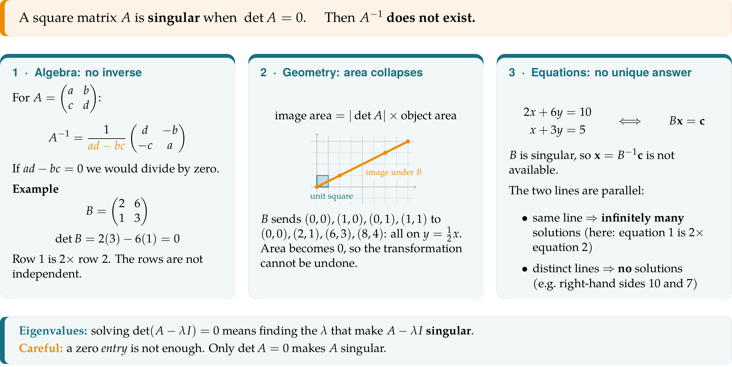
Core Concept The One-Way Shredder: Permanent Loss of Information
In everyday arithmetic, multiplying by zero is the classic operation that cannot be undone:
\[x \times 0 = 0\]Once you multiply by zero, you cannot ask "What was \(x\)?" because every number multiplied by zero produces zero. The original value of \(x\) is erased.
A singular matrix is the matrix equivalent of multiplying by zero. A non-singular matrix is a reversible machine: every output point comes from exactly one input point, so \(A^{-1}\) can run time backwards. A singular matrix is a shredder: it collapses different inputs into the exact same output, destroying information forever.
Watch what happens when the singular matrix \(B = \begin{pmatrix} 2 & 6 \\ 1 & 3 \end{pmatrix}\) acts on two completely different starting points: \[B \begin{pmatrix} 3 \\ 0 \end{pmatrix} = \begin{pmatrix} 2(3) + 6(0) \\ 1(3) + 3(0) \end{pmatrix} = \begin{pmatrix} 6 \\ 3 \end{pmatrix}\] \[B \begin{pmatrix} 0 \\ 1 \end{pmatrix} = \begin{pmatrix} 2(0) + 6(1) \\ 1(0) + 3(1) \end{pmatrix} = \begin{pmatrix} 6 \\ 3 \end{pmatrix}\]
Both \((3, 0)\) and \((0, 1)\) collide into the exact same destination \((6, 3)\)! If someone hands you the output \(\begin{pmatrix} 6 \\ 3 \end{pmatrix}\) and asks "What was the input vector?", you cannot answer. Was it \((3, 0)\)? \((0, 1)\)? Or \((-3, 2)\)? The information has been permanently destroyed.
Why this kills the inverse: A mathematical function can only assign one output to each input. An inverse matrix \(B^{-1}\) would have to map that single point \((6, 3)\) back to infinite different starting points simultaneously. That is impossible. Once information is destroyed, no matrix can retrieve it.
Visual Checklist How to Spot a Singular Matrix at a Glance
The determinant is your official mathematical test: a matrix is singular if and only if \(\det A = 0\). But for a \(2 \times 2\) matrix you can often spot singularity in a couple of seconds without a full calculation:
1. The Diagonal Balance (\(ad = bc\))
For any \(2 \times 2\) matrix \(\begin{pmatrix}a & b \\ c & d\end{pmatrix}\):
\[\det A = ad - bc = 0 \iff \mathbf{ad = bc}\]
Multiply the main diagonal (\(a \times d\)) and off-diagonal (\(b \times c\)). If the two products are equal, \(\det = 0\) instantly! (e.g. \(\begin{pmatrix}4 & 6 \\ 2 & 3\end{pmatrix} \to 4\times 3 = 12\) and \(6\times 2 = 12\)).
2. Multiples in the Rows
One row is a direct scalar multiple of another:
\[\begin{pmatrix} 2 & 6 \\ 1 & 3 \end{pmatrix} \implies \text{Row 1} = 2 \times \text{Row 2}\]
If one row is proportional to another, the two equations tell you the exact same thing. One equation is redundant, leaving you with insufficient constraints to solve the system.
3. Multiples in the Columns
One column is a direct scalar multiple of another:
\[\begin{pmatrix} 2 & 6 \\ 1 & 3 \end{pmatrix} \implies \text{Col 2} = 3 \times \text{Col 1}\]
Columns represent where basis vectors \(\mathbf{i}\) and \(\mathbf{j}\) land. If Column 2 is parallel to Column 1, both basis vectors land on the same 1D line, collapsing 2D area to zero!
4. Any Row or Column of Zeros
If an entire row or column consists solely of zeros:
\[\begin{pmatrix} 0 & 0 \\ 5 & -3 \end{pmatrix} \text{ or } \begin{pmatrix} 7 & 0 \\ 4 & 0 \end{pmatrix}\]
The determinant is zero immediately because one direction has been completely wiped out, squashing all space flat.
1 · Geometry The Collapse of Dimension
In section 5.3, we saw that the determinant represents the signed area scale factor of a 2D transformation:
\[\text{area of image} = |\det A| \times \text{area of object}\]If \(\det A = 0\), the image area of every possible shape is multiplied by zero. What 2D shape has zero area?
A flat 1D line (or a single point at the origin).
The columns of a matrix tell you where the unit basis vectors \(\mathbf{i} = \begin{pmatrix}1\\0\end{pmatrix}\) and \(\mathbf{j} = \begin{pmatrix}0\\1\end{pmatrix}\) land. When the columns are multiples of each other, those two landing vectors point in the exact same line. They cannot form a 2D parallelogram; they can only span a 1D line!
Why this kills the inverse: Whole sets of different points are squashed onto the same single image point (for \(B\), the points \((3,0)\), \((0,1)\) and \((-3,2)\) all land on \((6,3)\)). An inverse would have to map that one point back to infinitely many different points, which is impossible for a function. The transformation is strictly one-way.
2 · Algebra Dividing by Zero is Just the Symptom
For a standard \(2\times 2\) matrix:
\[A = \begin{pmatrix} a & b\\ c & d\end{pmatrix},\qquad \det A = ad-bc\]the algebraic formula for the inverse is:
\[A^{-1} = \frac{1}{\det A}\begin{pmatrix} d & -b\\ -c & a\end{pmatrix} = \frac{1}{ad-bc}\begin{pmatrix} d & -b\\ -c & a\end{pmatrix}\]If \(ad - bc = 0\) (or \(ad = bc\)), the formula divides by zero. But this division by zero isn't an arbitrary mathematical accident:
To inflate a 1D line of zero thickness back into a 2D plane with area, you would need an infinite area expansion factor (\(\frac{1}{0}\)). The algebra is simply reporting the geometric reality: you cannot stretch a line into a plane with a finite matrix.
Linear Dependence: Look at the rows and columns of \(B = \begin{pmatrix} 2 & 6 \\ 1 & 3 \end{pmatrix}\):
- Row 1 is exactly \(2 \times\) Row 2.
- Column 2 is exactly \(3 \times\) Column 1.
A matrix is singular whenever its rows (or columns) are linearly dependent—meaning one vector is redundant and adds no new dimension.
3 · Applied Systems Redundant Information
Consider setting up a system of simultaneous equations from a real-world scenario:
"At the cafe, 2 coffees and 6 pastries cost €20."
"Later, 1 coffee and 3 pastries cost €10."
If we write this as a matrix system \(B\mathbf{x} = \mathbf{c}\):
\[\begin{pmatrix} 2 & 6 \\ 1 & 3 \end{pmatrix}\begin{pmatrix} c \\ p \end{pmatrix} = \begin{pmatrix} 20 \\ 10 \end{pmatrix}\]Can you determine the price of a coffee? No. Statement 2 provides zero new information—it is literally statement 1 divided by 2. Because the matrix is singular:
- Coincident lines: Infinitely many combinations of coffee and pastry prices work (e.g., \(c=4, p=2\) or \(c=1, p=3\)).
- Parallel inconsistent lines: If the second receipt had claimed €12, the equations would contradict each other, yielding no solution.
A singular matrix in a model is a red flag: it means your measurements contain redundant variables or conflicting constraints.
The Grand Twist The Secret Weapon for Eigenvalues
In sections 5.4 and 5.5, singularity seems like a nuisance—a breakdown of the inverse tool.
Then comes AHL 5.6: Eigenvalues and Eigenvectors. Here, singularity becomes our most celebrated technique.
An eigenvector \(\mathbf{v}\) is a vector whose direction is unchanged by matrix \(A\), merely scaled by \(\lambda\):
\[A\mathbf{v} = \lambda\mathbf{v} \quad\iff\quad (A - \lambda I)\mathbf{v} = \mathbf{0}\]Notice what this equation says: we are looking for a non-zero vector \(\mathbf{v}\) that gets sent to \(\mathbf{0}\).
- If \((A - \lambda I)\) were non-singular, it would have an inverse. Multiplying by \((A - \lambda I)^{-1}\) would give \(\mathbf{v} = \mathbf{0}\)—the useless trivial answer.
- To get real, non-zero eigenvectors, the matrix \((A - \lambda I)\) MUST collapse space! It must squash a whole line of vectors down to the origin.
That is why we solve the characteristic equation:
\[\det(A - \lambda I) = 0\]We are deliberately hunting for the values of \(\lambda\) that make the matrix singular! What started as a flaw in 5.4 becomes the exact key that unlocks Google's PageRank, quantum states, and structural vibration modes.
AI HL Where it matters in AI HL
- Inverses and systems. Check the matrix is non-singular before using \(A^{-1}\). For a \(2\times 2\) matrix, find \(\det A\) by hand first; for larger matrices use your GDC. On the TI-Nspire, trying to invert a singular matrix gives an error rather than an answer.
- Eigenvalues. You find them by solving \(\det(A-\lambda I)=0\). That is, you look for the values of \(\lambda\) that make \(A-\lambda I\) singular. Singularity is exactly what allows a non-zero eigenvector \(\mathbf{v}\) with \((A-\lambda I)\mathbf{v}=\mathbf{0}\).
Summary: Singular vs. Non-Singular
| Property | Singular Matrix (\(\det A = 0\)) | Non-Singular Matrix (\(\det A \neq 0\)) |
|---|---|---|
| Inverse | Does not exist (\(A^{-1}\) undefined) | Unique inverse exists |
| Geometric effect | Collapses 2D area to a 1D line or point | Preserves dimension; scales area by \(|\det A|\) |
| Linear system \(A\mathbf{x}=\mathbf{b}\) | No unique solution (either infinite or none) | Unique solution: \(\mathbf{x} = A^{-1}\mathbf{b}\) |
| Rows & Columns | Linearly dependent (redundant information) | Linearly independent (full dimension) |
| Role in Eigenvalues | The goal! \(\det(A - \lambda I) = 0\) gives the eigenvalues, and allows non-zero eigenvectors | Yields only the trivial zero vector \(\mathbf{v}=\mathbf{0}\) |
Check Your Understanding
1. Given \(M = \begin{pmatrix} 2 & k \\ 5 & -15 \end{pmatrix}\), find \(k\) such that \(M\) is singular, and write the equation of the line that space collapses onto.
Step 1: Set \(\det M = 0\).
\[\det M = (2)(-15) - (k)(5) = -30 - 5k = 0 \implies 5k = -30 \implies k = -6\]Step 2: Find the collapsed line.
The columns are \(\begin{pmatrix} 2 \\ 5 \end{pmatrix}\) and \(\begin{pmatrix} -6 \\ -15 \end{pmatrix} = -3\begin{pmatrix} 2 \\ 5 \end{pmatrix}\). Both vectors lie along the line through the origin with gradient \(m = \frac{5}{2} = 2.5\).
Therefore, the entire 2D coordinate plane is squished onto the line \(y = \frac{5}{2}x\) (or \(5x - 2y = 0\)).
2. An engineering model sets up a system \(C\mathbf{x} = \mathbf{d}\) with 3 alloys. The calculator returns \(\det C = 0\). What does this tell the engineer?
A determinant of zero means the 3 alloy equations are not linearly independent. One alloy mixture's recipe is a linear combination of the other two, providing no new constraint.
Depending on the target vector \(\mathbf{d}\), the engineer either has infinitely many recipes that meet the specification, or the specification is contradictory and no recipe is possible. Either way there is no unique answer, and \(C^{-1}\) cannot be used.
3. For \(A = \begin{pmatrix} 4 & 1 \\ 2 & 3 \end{pmatrix}\), why does solving \(\det(A - \lambda I) = 0\) find the eigenvalues?
We require \((A - \lambda I)\mathbf{v} = \mathbf{0}\) to have non-zero solutions for \(\mathbf{v}\).
If \((A - \lambda I)\) were non-singular, its inverse would force \(\mathbf{v} = (A - \lambda I)^{-1}\mathbf{0} = \mathbf{0}\). Thus, we require \((A - \lambda I)\) to be singular so that a whole line of non-zero vectors gets collapsed onto \(\mathbf{0}\).
\[\det\begin{pmatrix} 4-\lambda & 1 \\ 2 & 3-\lambda \end{pmatrix} = (4-\lambda)(3-\lambda) - 2 = \lambda^2 - 7\lambda + 10 = (\lambda - 2)(\lambda - 5) = 0\]The matrix becomes singular precisely when \(\lambda = 2\) or \(\lambda = 5\). Along these special eigenvector directions, \(A\) acts as a pure scalar stretch of factor 2 or 5.
See also: Where are eigenvectors used? (AHL 5.6, extension).
IBDP AI HL · Matrices · J. Murphy · jmaths.xyz